Where should each layer live?
When one GPU is too small or too slow for a model, you spread the model over several. Then you have to decide which layer goes on which card. Put two layers that talk a lot on different cards and every step pays for copying data between them. Pile everything on one card and the others sit idle. People usually make this call by hand, with rules of thumb.
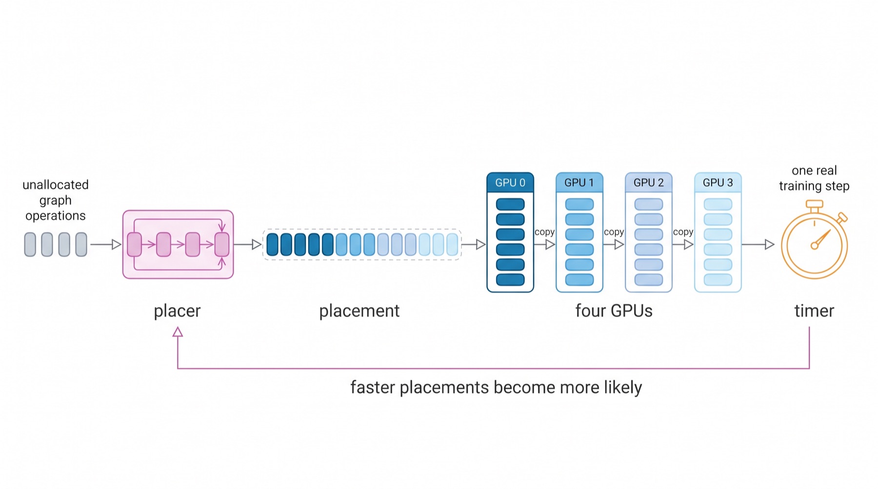
In 2017, Azalia Mirhoseini and colleagues at Google Brain asked whether a network could learn this decision instead. Their placer reads the model's computation graph and writes down a device for every operation. The only feedback it gets is how long one training step took. They showed it could find placements faster than expert-designed ones on Inception-V3, a recurrent language model and a translation model. Mirhoseini later co-led AlphaChip and co-founded Ricursive Intelligence, a lab built on the same instinct: let AI design the hardware side of AI.
This post rebuilds that experiment small enough to run in an afternoon: a 49M-parameter GPT, four NVIDIA T4s on Modal, and roughly $20 of GPU time. Every number below comes from real runs and was re-measured in a separate head-to-head test.
The game: 40 decisions, 4 GPUs
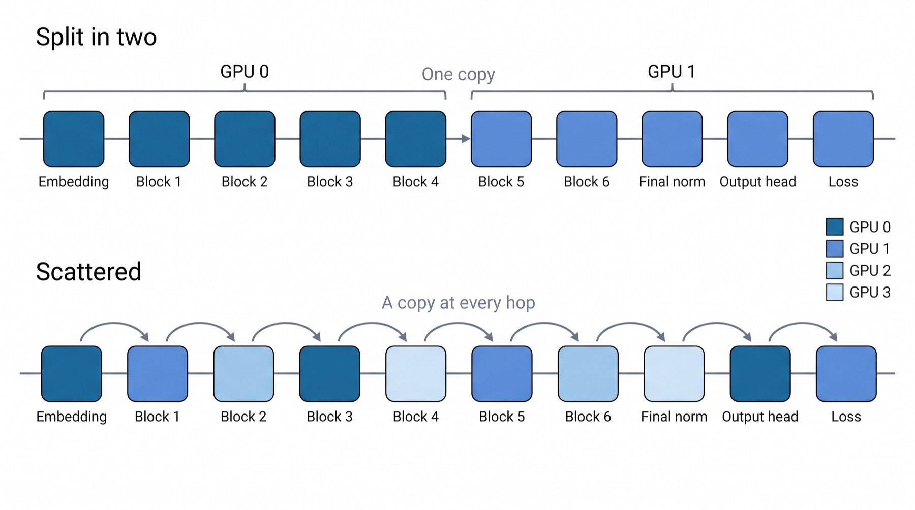
PyTorch has no fixed graph to place, so we wrote the GPT as an explicit chain of 40 placeable nodes: the embedding, six transformer blocks of six nodes each (layer norm, attention, residual add, layer norm, MLP, residual add), then the final norm, the output head and the loss. The model has 49M parameters. 39M of them sit in just two nodes, the embedding and the output head, because the vocabulary has 50,257 tokens.
A placement is one GPU index per node, so there are 440 of them. The environment runs a real training step under the placement (forward, backward and an AdamW update on a batch of 16 × 256 tokens), copying activations whenever an edge crosses GPUs. Its reward is the median wall-clock time of 5 steps after 2 warm-up steps. A placement that runs out of memory is charged 10 seconds.
The placer and REINFORCE
The placer follows the paper. Each node is described by three things: its operation type, the shape of its output and which nodes it connects to. An encoder LSTM reads the nodes in order. A decoder LSTM then walks the same sequence and picks a GPU for each node. At every step it looks back over all the encoder states (attention) and sees which GPU it chose for the previous node.
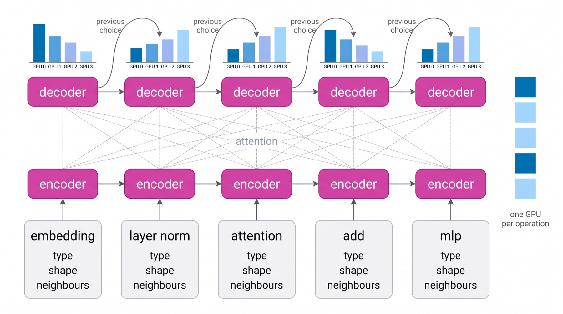
Training is REINFORCE, as in the paper. Each update samples 8 placements and times all of them. Each placement's cost is the square root of its step time, which squashes the huge gap between terrible and decent placements. The update raises the probability of placements that cost less than a baseline and lowers the rest:
The paper's baseline is a moving average of past costs. That is the version we started with.
It learns in ten updates, then stops
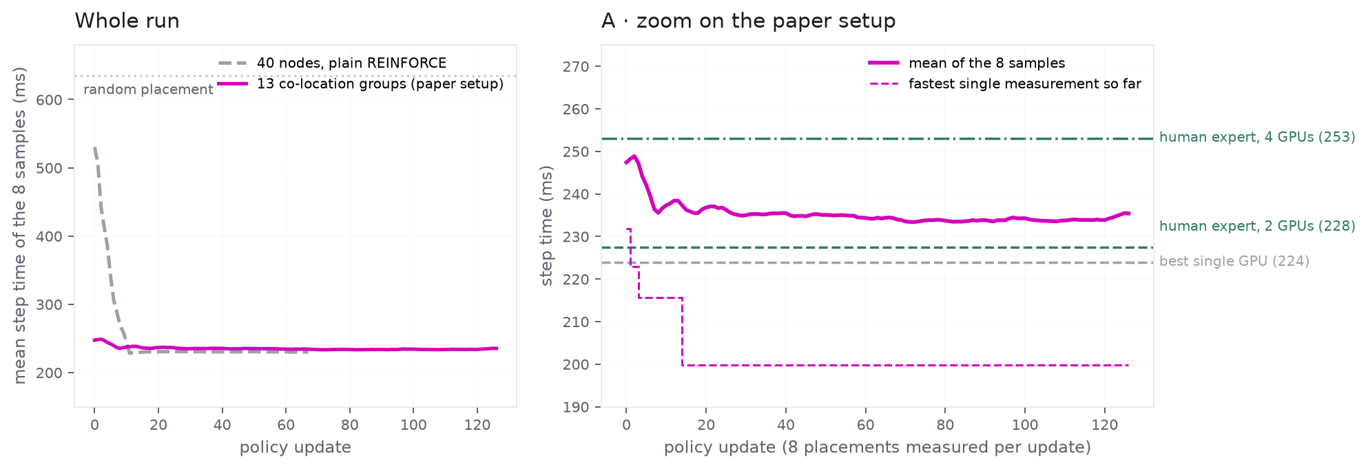
The first run was encouraging for about thirty seconds of reading. The mean step time of the sampled placements fell from 530 ms to 230 ms in eight updates. By update sixteen, all eight samples in every batch were the same placement: everything on one GPU. When every sample is identical, every sample gets the same score, the update is zero, and learning is over for good.
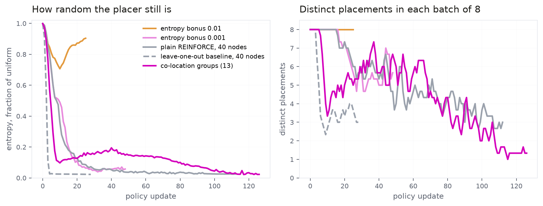
We tried three standard fixes before understanding the real problem:
- An entropy bonus, which rewards the placer for staying uncertain. At 0.01 it stayed almost uniform, and its samples kept averaging 450 to 490 ms. At 0.001 it collapsed a little later than without.
- A leave-one-out baseline. We suspected the moving average lagged behind a fast-improving policy, so that every sample looked "better than average" and got reinforced. Comparing each sample with its seven batch-mates removes that effect. At the same learning rate it collapsed even faster, within about five updates.
- A lower learning rate only slowed the same slide.
The real cause is in the placements themselves. "Put this node on the same GPU as the one before it" is right almost everywhere, so the placer learns it at all 40 decisions at once and becomes nearly deterministic. From there, a better placement needs several decisions to change together. The clearest case is the output head and the loss: moving only one of them forces the 823 MB logits tensor (16 × 256 × 50,257 floats) across the PCIe bus, which is much slower. One-node-at-a-time exploration can't climb over that wall.
The paper's own fix: co-location groups
The paper does not place every operation separately. It first merges operations that obviously belong together and places the groups. We used the simplest rule of that kind: an operation whose output has exactly one consumer joins its consumer's group. On our GPT this turns 40 nodes into 13 groups: the embedding, two groups per transformer block, and a final group that holds the last MLP, the final norm, the output head and the loss.
The wall disappears, because head and loss now move together. The search space shrinks from 440 to 413, and even the very first random batch averages 247 ms instead of 530 ms. The placer still settles eventually, but it explores for about a hundred updates first, and that is long enough.
Results: two wins and a loss
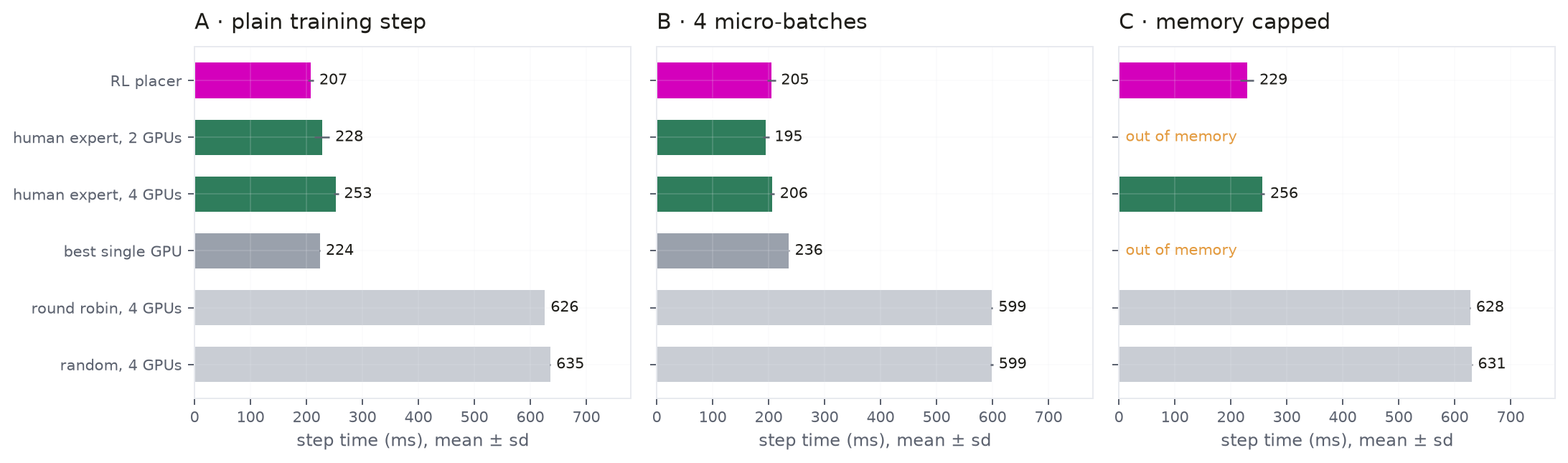
A single timing of a multi-GPU placement can be off by 5 to 15 ms, and the fastest timing out of two thousand is always flattered by luck. So every result below comes from a separate head-to-head test on one machine. In 4 shuffled selection rounds we pick the best RL placement (from the training run's top 5 and its final favourite), the best single GPU (out of 4) and the best two-GPU human split (on three GPU pairs). Then 8 fresh confirmation rounds time only those picks and the fixed baselines. Only confirmation numbers are reported, and every side gets exactly one pick.
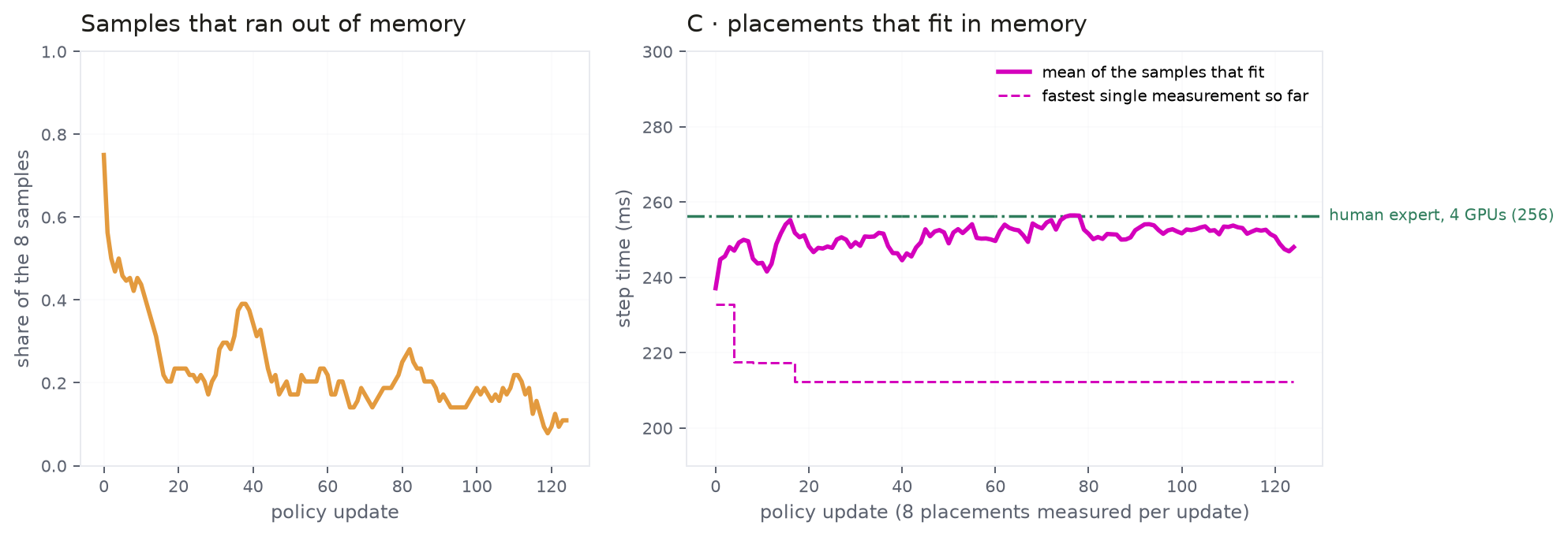
We ran three settings. A is a plain training step. B splits each batch into 4 micro-batches, so GPUs can work on different micro-batches at once, like an assembly line. C caps every GPU at 24% of its memory, so the model no longer fits on one card, the situation the paper was written for.
| Placement | A · plain | B · micro-batches | C · memory capped |
|---|---|---|---|
| RL placer | 207.4 ± 5.5 | 205.0 ± 7.1 | 229.2 ± 12.1 |
| Human expert, 2 GPUs (best pair) | 227.5 ± 13.8 | 195.3 ± 5.2 | out of memory |
| Human expert, 4 GPUs | 253.1 ± 3.9 | 206.3 ± 3.7 | 256.3 ± 4.0 |
| Best single GPU | 223.9 ± 0.5 | 236.2 ± 0.6 | out of memory |
| Round robin, 4 GPUs | 625.6 | 598.7 | 627.6 |
| Random, 4 GPUs | 635.3 | 598.7 | 631.1 |
| RL vs best alternative | −7.4% | +5.0% | −10.6% |
Step time in ms, mean ± standard deviation over 8 confirmation rounds of 10 timed steps each. The standard error of each mean is about a third of the standard deviation shown, so the A and C gaps are well outside the noise (about 8 and 6 standard errors). B is a clear loss.
Is A a lucky seed?
We trained three more A placers with different seeds and settings and gave each the same head-to-head test, on a different machine each time. All four beat every hand-made placement:
| A run | RL placer | Best single GPU | Best human split | Gain |
|---|---|---|---|---|
| 13 groups, moving average (paper setup) | 207.4 | 223.9 | 227.5 | −7.4% |
| 13 groups, leave-one-out, seed 0 | 213.7 | 232.7 | 223.9 | −4.6% |
| 13 groups, leave-one-out, seed 1 | 215.5 | 233.3 | 234.8 | −7.6% |
| 40 nodes, plain REINFORCE (the run that collapsed) | 213.1 | 229.8 | 235.1 | −7.3% |
Even the run that collapsed onto a single GPU had sampled the winning idea on its way down, which is why the paper reports the best placement found, not the policy's last guess.
Why the winning placement wins
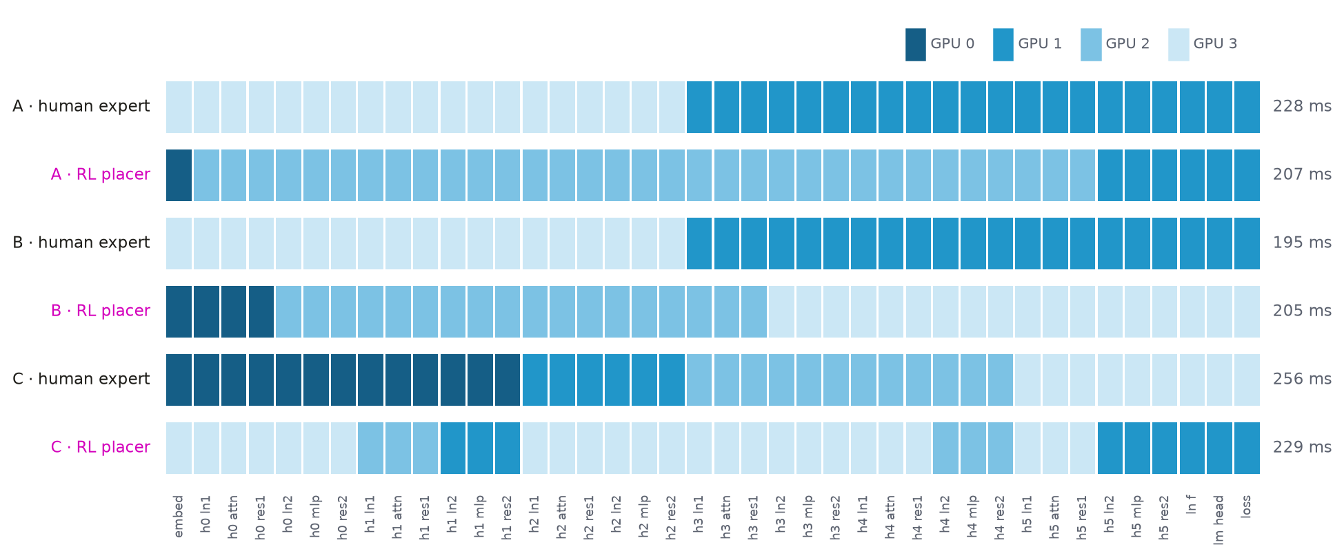
All four A runs found the same idea independently: keep the embedding and the output head away from the transformer body. Three of them use three GPUs (embedding, body, head). The fourth puts embedding and head together on one GPU and the body on another.
A GPT is a strict chain, so the forward and backward passes can't overlap across GPUs. So where does a 7% gain come from? We timed the three phases of a step separately, on one machine:
| Placement | Forward | Backward | Optimizer step | Total |
|---|---|---|---|---|
| Fastest single GPU | 70.1 | 135.9 | 17.1 | 223.1 |
| RL placer (A) | 67.9 | 136.9 | 8.0 | 212.9 |
Milliseconds, median of 12 steps, with every GPU synchronised between phases (so totals differ slightly from the head-to-head numbers).
The AdamW update is independent for every parameter, so it is the one part of a training step that can run on several GPUs at once. Putting the two vocabulary-sized layers on their own GPUs splits the 49M-parameter update three ways and more than halves its time, while forward and backward stay on the fastest card. The only extra traffic is two 6 MB activation copies each way.
None of the hand-made placements in this study does this, but once you see it, it makes sense. That may be the real value of the method: a search that turns up an idea a person can then understand and reuse. A human engineer would probably get the same speed-up today by sharding the optimizer state directly.
B: where the human wins
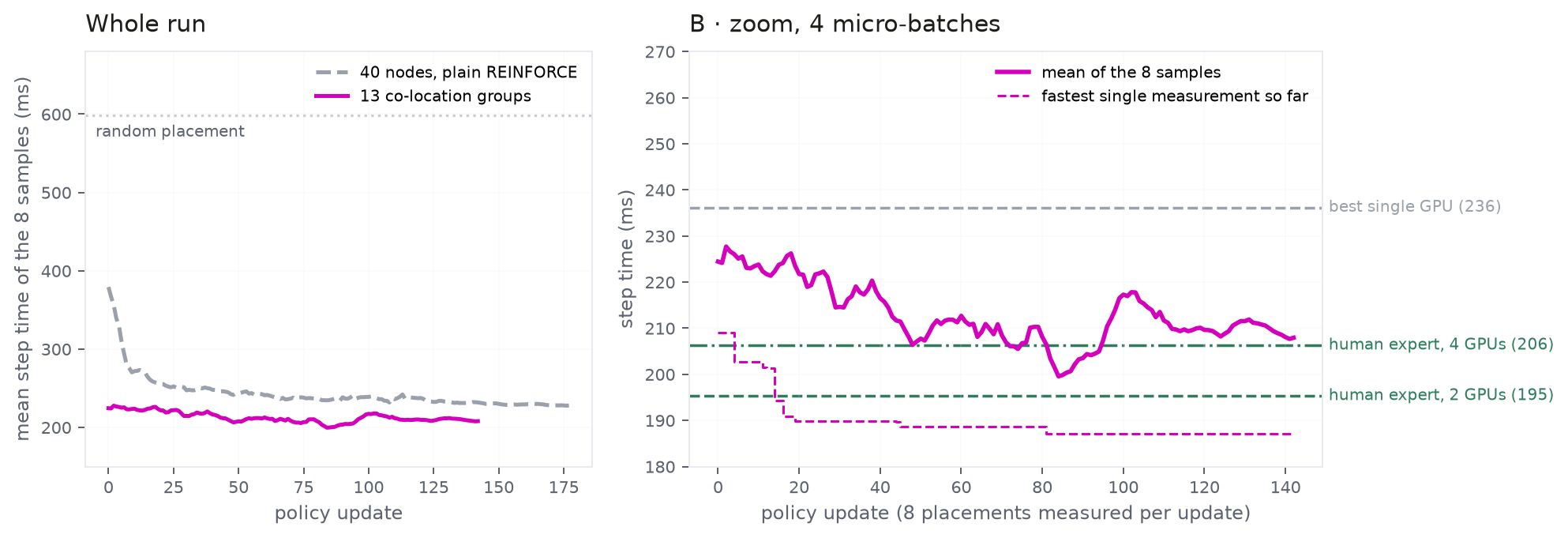
With 4 micro-batches, a clean two-stage pipeline lets GPU 3 work on micro-batch two while GPU 1 finishes micro-batch one. The human split (layers 1–3 on one GPU, layers 4–6 and the head on another) does that at 195 ms. The placer converged on a three-stage pipeline at 205 ms, about as fast as the human four-stage split (206 ms) but not the two-stage one. Its fastest single training measurement was 187 ms, which shows how much luck a best-of-2,000 number contains.
C: when the model doesn't fit
With every GPU capped at 24% of its memory, a single GPU and every two-GPU split run out of memory. The only hand-made placement that fits is the four-way layer split, at 256 ms. At first three in four sampled placements ran out of memory. The placer learned to avoid that and found a placement at 229 ms that keeps most of the model on one card and moves only what it must.
What to distrust
- The policy itself never beat a single GPU in A. Its favourite placement at the end of training ran at 226 to 235 ms. The wins come from the best placement the search found, which matches how the paper reports results. They are not from the final policy.
- Our first "human expert" number was lucky. The first quick measurement put the two-GPU split at 208 ms. Re-timed fairly, on four different machines, it is 224 to 235 ms, with a spread of about ±14 ms. Multi-GPU timings on these machines are noisy; single-GPU timings vary by under 1 ms.
- Best-of-many measurements flatter. The fastest timing seen in training was 8 to 15 ms better than the same placement re-timed. Every claim here uses re-timed numbers.
- The four GPUs are not identical, and it changes per machine. On one machine GPU 3 was the fastest; on the next it was the slowest. A placer partly learns the quirks of the machine it trained on. We gave every baseline the same freedom to pick its GPUs.
- Experiment C crashed at update 124 of 250 with a CUDA launch failure, most likely after about 200 out-of-memory recoveries. We used the 124 updates it logged and did not re-run it.
- We changed the recipe along the way (entropy bonus, then leave-one-out, then co-location) and stopped runs early once all 8 samples were identical, to save money. Every run, including the failed ones, is in the results folder.
- This is one small model on one kind of hardware. T4s talk over PCIe. On NVLink GPUs, or with a fused or sharded optimizer, the optimizer-splitting trick may be worth less or nothing.
Reproduce it
The code, every run log and the figure script are on GitHub under the MIT license. Everything runs on Modal (4 × T4 per job). A training run of 250 updates takes about an hour. A head-to-head evaluation takes about 12 minutes. All the runs in this post cost roughly $20.
git clone https://github.com/RajatDandekar/device-placement-rl && cd device-placement-rl
pip install modal && modal setup
# tests: placer, REINFORCE and infrastructure (CPU container)
modal run modal_app.py --task test
# baselines on 4x T4
modal run modal_app.py --task smoke --config tiny
# experiment A, paper setup: 13 co-location groups, moving-average baseline
modal run --detach modal_app.py --task train --n-iters 250 --lr 1e-3 --colocate
# B and C used --baseline leave_one_out, plus --n-micro 4 (B) or --mem-cap 0.24 (C)
# fair head-to-head (select 4 rounds, confirm 8), then every figure
modal run modal_app.py --task evaluate --run tiny_b16_m1_coloc_lr0.001_s0
modal run modal_app.py --task figures
Nothing on this page is hand-drawn from numbers. The three diagrams are concept sketches with no data in them. Every chart and table is generated by figures.py from the run logs, and one command regenerates them all.
Then break it
- Shard the AdamW state across GPUs by hand. Does the RL placement still win?
- Scale to the 163M-parameter config, where memory pressure is real without an artificial cap.
- Swap REINFORCE for PPO, or let the placer learn the groups too, as the 2018 hierarchical follow-up by the same group does.
- Train on one machine and evaluate on another, and measure how much of the gain is machine-specific.